Safety Warning:

When connecting the instrument to a power source, make sure the power outlet has a When connecting the instrument to a power source wire. If When connecting the instrument to a power source, the instrument’s casing may become charged with static or induced electricity, which could result in personal injury!

Electric Shock Hazard Take precautions against electric shock when operating, testing, or maintaining the instrument. Non-professionals must not open the chassis without authorization. If a professional needs to replace a fuse or perform other maintenance, be sure to unplug the power cord first and have another person present during the procedure.

Even after the power cord has been unplugged, the charge stored in the capacitor may still present a dangerous voltage; therefore, do not handle the device until it has been discharged.

Do not replace or adjust the instrument’s internal circuitry or components without authorization.

Electrical shock hazards may result from improperly removing or connecting the device under test during testing, as the voltage at the test terminals may cause serious injury or property damage!!! Never touch the test terminals directly with your hands under any circumstances.

Input power supply: Please use an input power supply that meets the power specifications for this instrument. Using an input power supply that does not meet these specifications may damage the instrument.

When replacing a fuse, be sure to use one of the same specifications.

Stay Away from Explosive Gases

Electronic instruments must not be used in environments containing flammable or explosive gases, nor in environments containing corrosive gases or dust, to avoid creating a hazard.

Other Safety Precautions: Do not apply any voltage or current to the test terminals of this instrument.

You must strictly observe all safety precautions at all times when operating or maintaining this instrument. Failure to observe these safety precautions and the warnings in this manual may not only affect the instrument’s performance but may also result in direct damage to the instrument and pose a risk to personal safety. The Company assumes no liability for any consequences resulting from failure to comply with these safety precautions.

Table of Contents

2. Introduction to Measurement Parameters and Scan Patterns of Ultrasonic Devices 4

3. LS70A Series Impedance Analyzer Operating Guide 10

4. LS80A Series Impedance Analyzer Operating Guide 20

5. LS90A Series Impedance Analyzer Operating Guide 28

6. User Guide for Impedance Analysis Software 36

6.6.2 “Scan-to-Draw” Settings 43

6.6.3 “Kp Formula” Settings 43

6.6.4 “Comparison Settings” Tab 44

6.6.5 “Slice Dimensions” Tab 44

6.6.6 “Qm Formula” tab 45

7. Frequently Asked Questions and Solutions 48

1. Introduction to the LS70A/LS80A/LS90A Series Impedance Analyzers

The LS70A/LS80A/LS90A series instruments are primarily used for testing piezoelectric components and equipment. They offer a cost-effective solution for measuring and analyzing piezoelectric components and equipment, allowing for quick and convenient evaluation and testing of the parameters and characteristics of piezoelectric components.

Traditional ultrasonic impedance analyzers require a computer running software to perform scanning and analysis functions. In contrast, the LS70A/LS80A/LS90 series ultrasonic impedance analyzers from LISUN not only offer computer-based scanning and analysis capabilities but also display the scanning results of piezoelectric devices directly on the instrument itself, eliminating the need for customers to configure a computer for each unit. This approach ensures testing efficiency while reducing testing costs. It represents yet another value-added solution that this product series offers customers in the field of piezoelectric testing. At the same time, the series’ excellent measurement accuracy, ultra-wide frequency range, and outstanding stability can meet the vast majority of measurement requirements for ultrasonic devices and materials.

The LS70A/LS80A/LS90 Series Ultrasonic Impedance Analyzers support multiple communication interfaces (RS232, USB-CDC, USB-TMC). Compared to traditional ultrasonic impedance analyzers that only support RS232 communication, users can connect the analyzer to a computer using just a single USB cable, eliminating the need to install a dedicated RS232 serial communication card on the computer.

Ultrasonic impedance analyzers are primarily used to measure the impedance characteristics of various ultrasonic devices, including piezoelectric ceramics, transducers, ultrasonic cleaners, ultrasonic ranging systems, ultrasonic motors, ultrasonic flow meters, ultrasonic flaw detectors, and all other devices that utilize ultrasound.

2. Introduction to Measurement Parameters and Scan Patterns of Ultrasonic Devices

2.1 Measurement Parameters

For piezoelectric devices, their impedance characteristics vary with frequency. While a fully accurate description of a piezoelectric device requires an extremely complex circuit network, selecting a relatively simple network (consisting of inductors, resistors, and capacitors) within the frequency range of interest can provide a fairly complete description of the device’s characteristics. Practice has shown that constructing the network using the inductors, resistors, and capacitors included in the network described below can effectively reproduce the desired network characteristics.

For typical piezoelectric devices, there are no other resonances in the frequency range far from a given resonant frequency. In the frequency range near this resonant frequency, the device can be modeled using a number of inductors, resistors, and capacitors; the corresponding equivalent circuit is shown in the figure below:

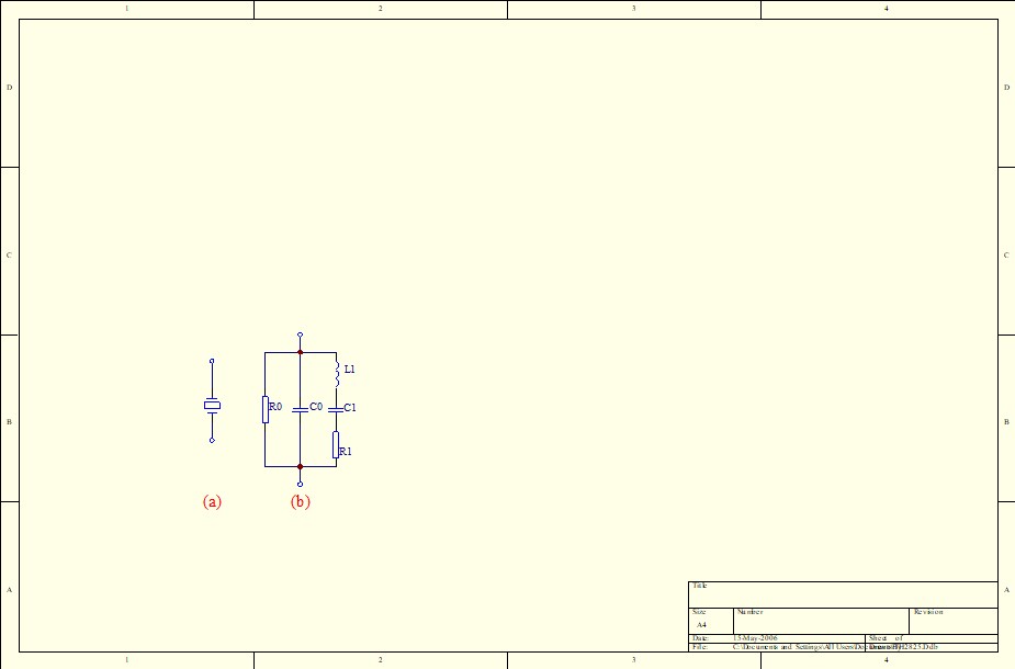
Figure 2-1: Equivalent Circuit Diagram of a Typical Piezoelectric Device

Figure 2-1(a) shows the symbol for a piezoelectric device, and Figure 2-1(b) shows its equivalent circuit. Here, C₀ is the static capacitance; R₁, C₁, and L₁ represent the resistance, capacitance, and inductance, respectively, in the dynamic impedance; and R₀ is the insulation impedance of the material.

In the equivalent circuit shown above, since the circuit is represented in parallel, it is more convenient to analyze it using admittance. Let the admittance of the entire circuit be Y, the admittance of the parallel branch (consisting of R0 and C0, referred to as the static admittance) be Y0, and the admittance of the series branch (consisting of R1, L1, C1, referred to as the dynamic admittance) as Y1.

Y = Y0 + Y1

Y0 = (1/R0) + j2πfC0,

Y1 = 1/(R1 + j2πf L1 + 1/(j2πf C1))

Through calculation, we can determine how the total admittance Y and the dynamic admittance Y1 vary with frequency f (admittance-frequency characteristics).

Y and Y1 are vectors; they must be decomposed into their real part (conductance G) and imaginary part (admittance B) in order to be represented graphically.

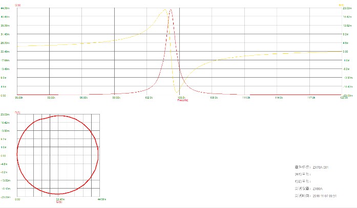
Figure 2-2: Admittance Characteristics of a Piezoelectric Device

Figure 2-2 shows two different representations of admittance characteristics. The upper half shows the frequency-dependent characteristics of conductance and admittance; the yellow line represents the B(S)–f characteristic, and the red line represents the G(S)–f characteristic. The lower half shows an admittance vector plane, where the horizontal axis represents conductance G (the real part of admittance) and the vertical axis represents admittance B (the imaginary part of admittance). This figure illustrates how the device’s admittance varies with frequency.

When the signal frequency varies within a range near the resonant frequency (series resonance), the trajectory of vector Y1 forms a circle with center at (1/2R1, 0) and radius 1/2R1.

When the trajectory of vector Y1 completes one full rotation around the resonance frequency, the variation of vector Y0 with frequency is generally small, so it can essentially be regarded as a constant. Therefore, by translating the trajectory of Y1 upward along the vertical axis in the admittance plane, we obtain the trajectory of admittance Y as a function of frequency—the so-called admittance circle.

Using this admittance plot, one can determine the equivalent circuit of the piezoelectric device and other important parameters.

(1) Fs: Mechanical resonance frequency, which is the operating frequency of the vibrating system; in design, it should be as close as possible to the desired value. For cleaning machines, the higher the consistency of the transducer’s resonance frequency, the better. For plastic welding machines or ultrasonic processing, if the horn or mold is poorly designed, the transducer’s resonance frequency may deviate from the operating point.

(2) Gmax: The conductance at series resonance; the conductance value when the vibrating system is operating; it is the reciprocal of the dynamic resistance R1. Under identical mounting conditions, a higher value is better; Gmax = 1/R1. Generally, for cleaning or welding transducers, this value ranges from approximately 50 mS to 500 mS. If the value is too low, the transducer or vibration system will typically experience issues, such as circuit mismatch, low conversion efficiency, or a shortened transducer lifespan.

(3) C0: The capacitance of the static branch in the equivalent circuit of a piezoelectric device; C0 = CT – C1 (where CT is the free capacitance at 1 kHz, and C1 is the capacitance of the dynamic branch in the equivalent circuit of the piezoelectric device). When using the device, C₀ must be balanced using inductors. In the circuit design of cleaning machines or ultrasonic processing equipment, properly balancing C₀ can improve the power factor of the power supply. There are two methods for balancing C₀ using inductors: parallel tuning and series tuning.

(4) Qm: Mechanical quality factor, determined using the conductance curve method; Qm = Fs / (F2 – F1). A higher Qm value is better because it indicates higher oscillator efficiency; however, Qm must be matched to the power source, and if the Qm value is too high, the power source cannot be matched.

When it comes to cleaning resonators, the higher the Qm value, the better. Generally speaking, the Qm value of a cleaning resonator should be 500 or higher; if it is too low, the resonator’s efficiency will be poor.

In ultrasonic machining, the Qm value of the transducer itself is generally around 500; when combined with the horn, it typically reaches around 1000; and when combined with the die, it generally reaches 1500 to 3000. If the Qm is too low, vibration efficiency is reduced; however, it should not be too high, because the higher the Qm, the narrower the operating bandwidth, making it difficult to match the power supply. Consequently, the power supply cannot operate at the resonant frequency, and the equipment will not function.

(5) F2, F1: Frequencies at the half-power points of the oscillator.

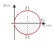
Looking at the admittance circle (shown below), the frequency at which the real part of the admittance equals Gmax/2 is determined. There are two such frequencies: F2, which is greater than Fs, and F1, which is less than Fs. F2 and F1 are then calculated using linear interpolation.

For the entire vibration system of an ultrasonic processing setup (including the horn and die), the difference between F2 and F1 must be greater than 10 Hz; otherwise, the frequency band will be too narrow, making it difficult for the power supply to operate at the resonant frequency, and the equipment will not function.

F2 – F1 is directly related to Qm, where Qm = Fs / (F2 – F1).

(6) Fp: Antiresonance frequency (primarily caused by resonance between C0 and L1); the resonance frequency of the parallel branch containing the piezoelectric oscillator. At this frequency, the impedance of the piezoelectric oscillator is at its maximum, and its admittance is at its minimum.

(7) Zmax: Anti-resonance impedance. Under normal conditions, the anti-resonance impedance of a transducer is typically several tens of kiloohms or higher. If the anti-resonance impedance is relatively low, the transducer’s service life is often shorter.

(8) CT: Free capacitance—the capacitance value of the piezoelectric device at a frequency of 1 kHz; this value matches that measured by a digital capacitance meter. Subtracting the dynamic capacitance C1 from this value yields the true static capacitance C0. C0 must be balanced using an external inductor, while C1 participates in energy conversion during system operation and does not require balancing.

(9) Dynamic resistance R1: This is the resistance in the series branch of the piezoelectric oscillator shown in the figure. The calculation formula is: R1 = 1/D, where D is the diameter of the admittance circle.

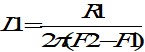
(10) Dynamic inductor L1: This is the inductor in the series branch of the piezoelectric oscillator shown in the figure.

The calculation formula is: , where R1 is the dynamic resistance, and F1 and F2 are the half-power points.

(11) Dynamic capacitor C1: This is the capacitor in the series branch of the piezoelectric oscillator shown in the figure.

The calculation formula is: , where Fs is the resonant frequency and L1 is the dynamic inductance.

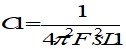
(12) Static capacitance C0: The calculation formula is C0 = CT – C1, where CT is the free capacitance and C1 is the dynamic capacitance.

(13) Keff: Effective electromechanical coupling coefficient. Generally speaking, the higher the Keff value, the higher the conversion efficiency. The formula is as follows:

(14) Free dielectric constant: This parameter applies only to piezoelectric ceramic discs. The calculation formula is as follows.

C is the free capacitance, in pF; t is the thickness of the wafer, in mm; A is the area of the wafer, in mm².

2.2 Scanning Graphics

Ultrasonic impedance analysis software can generate the following coordinate plots:

Admittance Coordinate System: GBF Coordinate Curves

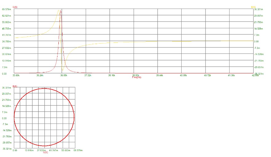
Upper graph: Red —— admittance real part G, Yellow —— admittance imaginary part B, Y-axis —— frequency

Lower half of the graph: Horizontal axis—real part of admittance (G); vertical axis—imaginary part of admittance (B).

Curves in the RXF Coordinate System for Impedance

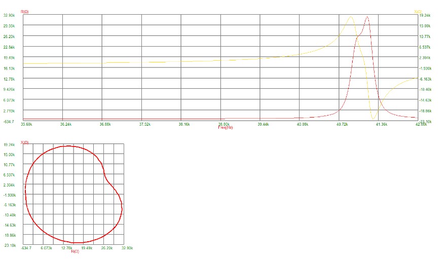
Upper graph: Red —— real part of impedance (R); Yellow —— imaginary part of impedance (X); Y-axis —— frequency

Lower half of the graph: Horizontal axis—real part of impedance (R); vertical axis—imaginary part of impedance (X).

Impedance in Polar Coordinates: Zθ-F Curve

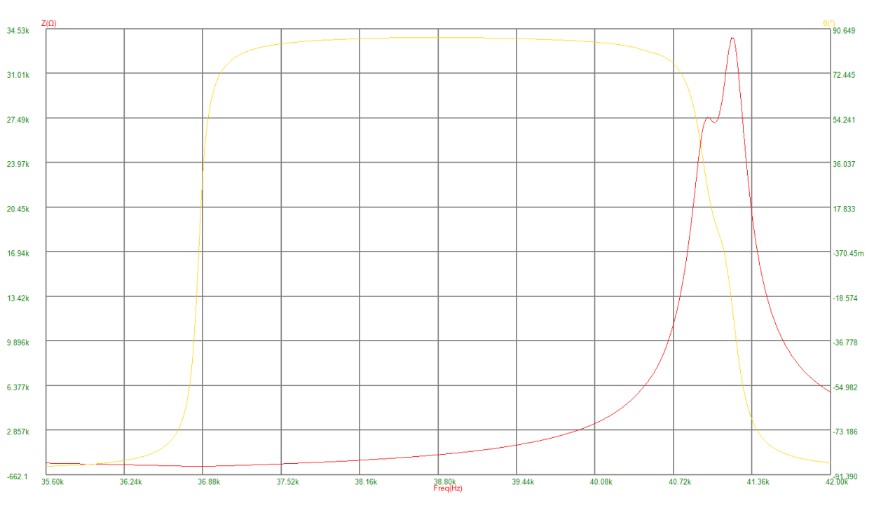
Red—impedance modulus |Z|, Yellow—impedance phase, Y-axis—frequency

Admittance in Polar Coordinates: Y(θ) vs. F Curve

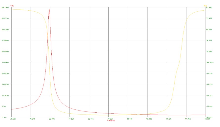
Red—–Admittance modulus |Y|, Yellow—-Admittance phase, Y-axis—-Frequency

Logarithmic coordinate system

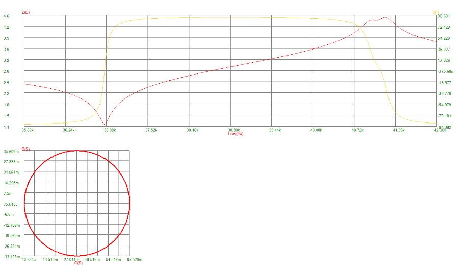
Upper section: Red—logarithm of the impedance modulus (lg|Z|); Yellow—impedance phase; Y-axis—frequency

Lower half: Horizontal axis—real part of admittance G; vertical axis—imaginary part of admittance B

3. LS70A Series Impedance Analyzer Operating Guide

3.1 Instrument Front Panel

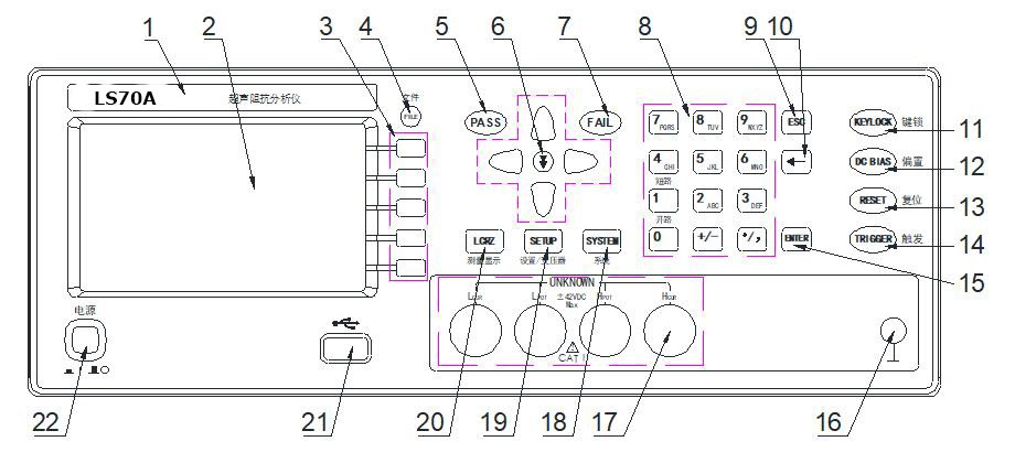
Figure 3-1 LS70A Front Panel

Brands and Models

Instrument Brand and Model Number

LCD Display

480×272 dot-matrix LCD display that shows setup information, measurement results, measurement conditions, and more.

Soft Keys

Five soft keys are available for selecting controls and parameters; the function of each soft key is defined to the left of it. The soft key definitions vary depending on the display page.

[FILE] Keyboard Shortcuts

Press the [FILE] key to go directly to the file screen.

PASS LED

The test results are indicated by an LED light.

NEXT button

Quick Page-Turn Keys

FAIL LED

The test failed due to the LED light.

Number Keys

Used to enter numbers and other relevant information.

ESC key

Finish entering the numbers on the numeric keypad.

[←] key

The BACKSPACE key. Press this key to delete the last character of the entered value.

KEYLOCK Key

Press the [KEYLOCK] button; the [KEYLOCK] indicator will light up, indicating that the panel buttons are currently locked. Press the [KEYLOCK] button again, and the [KEYLOCK] button will turn off, indicating that the keypad lock has been released. If the password function is set to “ON,” you must enter the correct password to release the keypad lock; otherwise, the keypad lock cannot be released.

When the instrument is under bus control (such as USBTMC), the [KEYLOCK] button will light up. Press the [KEYLOCK] button again, and it will turn off, indicating that the instrument has returned to local mode and the keyboard lock has been released.

[DC BIAS] button (LS70A series does not have a bias function)

The [DC BIAS] button is used to enable or disable the DC bias output. When you press the [DC BIAS] button, the [DC BIAS] indicator lights up, indicating that the DC bias output is enabled; Press the [DC BIAS] key again, and the [DC BIAS] indicator will turn off, indicating that DC bias output is disabled. On certain non-test screens where DC bias cannot be applied, pressing this key will have no effect.

[RESET] button (LS70A series does not have a bias function)

[TRIGGER] key

When the instrument’s trigger mode is set to MAN (Manual), press this key to trigger the instrument to perform a test.

[ENTER] key

When entering values, press the [ENTER] key to finish entering data and to confirm and save the data displayed on the bottom line of the LCD.

When entering a filename, press the [ENTER] key to finish entering the filename, confirm it, and save the filename displayed on the bottom line of the LCD.

Chassis When connecting the instrument to a power source Terminal

This terminal is connected to the instrument housing. It can be used for a protective or shielding When connecting the instrument to a power source connection.

Test End (UNKNOWN)

Four-terminal test connector. Used to connect to a four-terminal test fixture or test cable for measuring the device under test.

High-side current drive (Hcur);

High-side voltage sampling (Hpot);

Low-end voltage sampling (Lpot);

Low-end current drive (Lcur).

[SYSTEM] Menu button

Press the [SYSTEM] button to access the “System Settings” page.

[SETUP] Menu Button

Press the [SETUP] button to enter the “Curve Scan Settings” page.

[LCRZ] Menu Key

Press the [LCRZ] key to enter the “Curve Scan Display” page.

USB Host Port

Used to connect a USB flash drive.

Power Switch (POWER)

Press this button to turn the power on or off.

3.2 Rear Panel of the Instrument

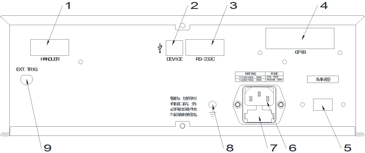
Figure 3-2: LS70A Rear Panel

HANDLER Interface

The HANDLER interface makes it easy to set up automated test systems and perform automated testing; it is widely used in automated factory production lines. The instrument uses this interface to output signals indicating the results of range comparisons and communication signals, and it also receives the “Start” signal through this interface.

USB DEVICE Port

The USBDEVICE interface allows a computer to control the instrument.

When the bus mode is set to USBTMC, this port functions as a USBTMC interface.

When the bus mode is set to USBCDC, this uses the USBCDC interface.

RS-232C Interface

Serial communication interface, which allows a computer to control the instrument.

GPIB Interface (Optional)

The GPIB interface enables parallel communication with a computer, allowing you to set up a GPIB test system.

220V/110V Switch

Used to switch between 110V and 220V AC input voltages.

For users in mainland China, the default AC input voltage is 220V; generally, there is no need to switch this switch.

Input power supply

For AC power input

Fuse

Used to install a power fuse to protect the instrument

When connecting the instrument to a power source Rod

This terminal is connected to the instrument housing. It can be used for a protective or shielding When connecting the instrument to a power source connection.

EXT. TRIG Interface

External Trigger Interface

3.3 Instrument Password

If the user set a startup password before the last shutdown, the instrument will prompt “Please enter the password:” upon startup. The default startup password for this instrument is: 2786.

3.4 Curve Scan Settings

Press the < SETUP> button to enter the “Curve Scan Settings” page, as shown in the figure below:

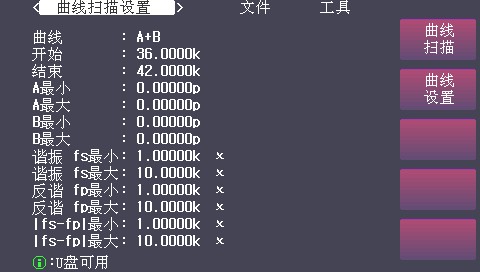
Figure 3-3: Curve Scan Settings Page

3.4.1 Curve Scan Parameter Settings

On the “Curve Scan” page, you can configure the following parameters:

Curve

A: Displays the main parameter curve during curve scanning

B: Display secondary parameter curves during curve scanning

A+B: Display both primary and secondary parameter curves simultaneously during curve scanning

Start

Set the Starting Scan Frequency

End

Set the Scan Completion Frequency

A (Minimum)

Set the minimum value for the main parameter

A is the largest

Set the maximum value for the main parameter

B is the smallest

Set the minimum value for the secondary parameter

B is the largest

Set the maximum value for the subparameter

Minimum resonant fs

Set the minimum resonance frequency

Maximum resonant fs

Set the Maximum Resonance Frequency

Minimize anti-resonance fp

Set the minimum anti-resonance frequency

Maximum anti-resonant fp

Set the maximum anti-resonance frequency

|fs – fp|minimum

Set the minimum difference between the positive and negative resonance points

|fs – fp|Maximum

Set the maximum difference between the forward and reverse resonance points

3.4.2 File Menu

File Management

Press this soft key to access the file management page, where you can save the configured parameters as a file for future use.

Screenshot

Press this soft key to copy the information on the screen to a USB flash drive.

3.5 Curve Scan Display

Press the < LCRZ> key to enter the “Curve Scan Display” page. As shown in the figure below:

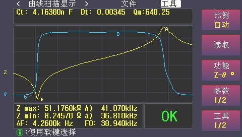
Figure 3-4: Curve Scan Display Page

The < Curve Scan Display> page performs automatic frequency-incremental scans of the device under test at 101201,401, or 801-point frequency intervals, in either linear or logarithmic mode. It dynamically displays on the LCD screen the response curves of the device’s primary and secondary parameters as they vary with frequency, and the measurement results for any point within the scan range can be read directly from the screen. It also displays the maximum and minimum measured values of the primary and secondary parameters for the component within the scan range, along with the corresponding test conditions.

The figure above shows the Z-Freq (yellow curve) and θ-Freq (blue curve) plots after the instrument has scanned a piezoelectric ceramic wafer (the horizontal axis represents frequency, and the vertical axis represents Z or θ).

A and a represent the points corresponding to the maximum and minimum values of impedance Z, respectively.

B and b represent the points corresponding to the maximum and minimum values of the phase angle θ, respectively.

Zmax represents the maximum value of impedance Z. A) The number on the right indicates the frequency corresponding to Zmax.

Zmin represents the minimum value of impedance Z. a) The number on the right indicates the frequency corresponding to Zmin.

The Ct on the graph represents the free capacitance, which is the capacitance value of the piezoelectric device at a frequency of 1 kHz. Dt represents the loss value of the piezoelectric device at a frequency of 1 kHz. Qm is the mechanical quality factor.

Note: After the user has set the scan conditions, they must press the [TRIGGER] button on the front panel to start the scan.

If you would like to obtain more parameters for piezoelectric devices, please install and run the “Impedance Analysis Software” on your computer. The main interface of the Impedance Analysis Software is shown below:

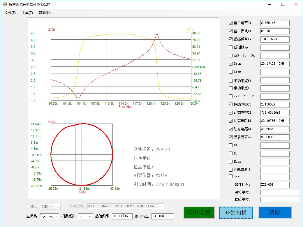
Figure 3-5: Main Interface of the Impedance Analysis Software

3.5.1 Common Menus for Curve Scanning

Move the cursor to “Tools,” and the instrument will display the commonly used curve scan menu, as shown below:

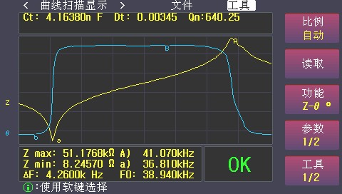
Figure 3-6: Common Menu for Curve Scanning 1

Ratio

Press this soft key to toggle between “Scale: Auto” and “Scale: Locked.”

Note: When “Scale: Locked” is selected, users must manually set parameters such as A Min, A Max, B Min, and B Max on the < Curve Scan Settings> page to adjust the display scale of the curve.

Read

When the “Read” button is pressed, “Read” appears in this area, indicating that the system is currently in data-reading mode.

Special Note: To view the measurement results for each condition point, follow these steps: Use the arrow keys on the panel. The [↓] key moves quickly toward the high end (right); the [↑] key moves quickly toward the low end (left); the [→] key moves one condition point at a time toward the high end (right); [←] moves one condition point at a time toward the lower end (left).

Features

Press this button to select different measurement parameters

Parameters

Press this key to switch between the primary and secondary parameters.

Tools 1/2

Press this key to switch to “Tool 2/2.”

Press the “Tool 1/2” soft key to switch to the “Tool 2/2” soft key menu. The menu is as follows:

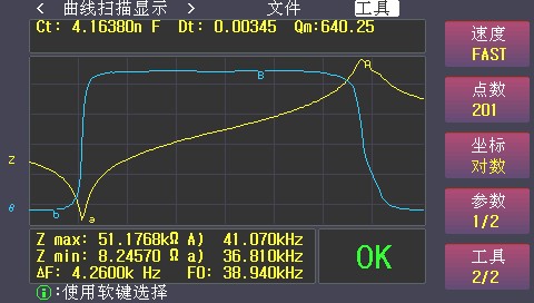
Figure 3-7: Common Menus for Curve Scanning 2

Speed

Press this button to switch between scan speeds: FAST, MED, and SLOW

Points

Press this button to cycle through scan points 101201, 401, and 801.

Coordinates

Press this soft key to switch between logarithmic and linear coordinates.

Parameters

Press this key to toggle between the primary and secondary parameters.

Tools 2 of 2

Press this key to switch to “Tool 2/2.”

3.5.2 File Menu

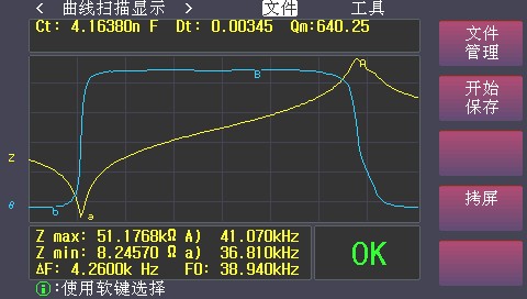
Figure 3-8: Curve Scan File Menu

File Management

Press this soft key to access the file management page, where you can save and load settings.

Start Saving

Press this button to save the scanned data to a USB flash drive.

Screenshot

Press this soft key to copy the information on the screen to a USB flash drive.

3.6 LS70A HANDLER Sorting Interface

The HANDLER sorting interface is located on the rear panel of the instrument; the pin assignments are shown in the figure below:

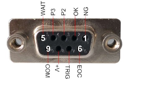
Figure 3-9 LS70A HANDLER Sorting Interface Pinout Diagram

The meanings and usage of the HANDLER port and pin assignments are as follows:

Pin Number	Signal Name	Signal Type	Signal Meanings
1	/NG	Output	Invalid signal, low active
2	/OK	Output	Valid signal, low active
3	/P2	Output	Reserved; the LS70A does not use this pin.
4	/P3	Output	Reserved; the LS70A does not use this pin.
5	/WAIT	Output	Instrument BUSY signal, active low. When this signal is active, it indicates that the instrument is performing a measurement or calculation.
6	/EOC	Output	Measurement Complete Signal, Low Active
7	/TRIG	Input	Triggers the instrument to take a measurement; low active. This signal is supplied externally to the HANDLER’s input.
8	EXTV+	Power Supply Positive Terminal	External Power Supply (High-Side)
9	COM	Negative Terminal of the Power Supply	0 V, lower limit of external power supply

4. LS80A Series Impedance Analyzer Operating Guide

4.1 Instrument Front Panel

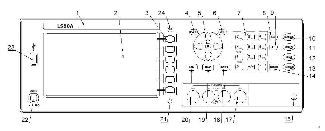
Figure 4-1: LS80A Front Panel

Brands and Models

Instrument manufacturer’s brand name and instrument model number.

LCD Display

Extra-large 800×480 dot-matrix LCD display that shows settings, measurement results, measurement conditions, and more.

Soft Keys

Soft keys are used to select parameters; the function of each soft key is defined to the left of the key. The soft key definitions vary depending on the display page.

PASS Light

The “PASS” light turns on when the test results are satisfactory.

NEXT button

This instrument does not use this key.

“FAIL” Light

If the test results are unsatisfactory, the “FAIL” light will illuminate.

Number Keys

Used to enter numbers.

ESC key

Exit button.

Backspace key

Backspace key

KEYLOCK

This indicator light turns on when the keyboard is locked. Press this key to lock or unlock the keyboard.

DC BIAS

This instrument does not use this key.

RESET button

This instrument does not use this key.

TRIG Key

Trigger button, used to initiate a measurement on the instrument.

ENTER key

Confirmation key, used to confirm after entering a number.

Chassis When connecting the instrument to a power source Terminal

This terminal is connected to the instrument housing. It can be used for protective or shielding When connecting the instrument to a power source connections.

None

Test End

The test end is used to connect to a four-terminal test fixture or test cable.

SYSTEM key

Press the SYSTEM key to enter the “System Settings” page.

SETUP button

Press the SETUP button to enter the “Measurement Settings” page.

LCRZ Key

Press the LCRZ key to enter the “Measurement Display” screen.

Return key

This instrument does not use this key.

Power Button

Press this button to turn the power on or off.

USB Host Port

For connecting a USB flash drive

FILE key

Keyboard shortcut to open the file management page.

4.2 Rear Panel of the Instrument

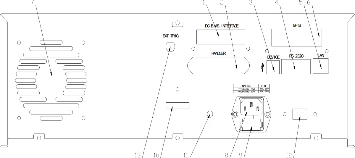
Figure 4-2: Rear Panel of the LS80A

DC BIAS Interface (for expansion)

HANDLER Port

The HANDLER interface makes it easy to set up automated test systems and perform automated testing, and is widely used in automated factory production lines. The instrument uses this interface to output range comparison results and communication signals, and simultaneously receives the “Start” signal through this interface.

USBDEVICE Interface

The USBDEVICE interface enables a computer to control the instrument.

When the bus mode is set to USBTMC, this port functions as a USBTMC interface.

When the bus mode is set to USBCDC, this port functions as a USBCDC interface (virtual serial port).

When the bus mode is set to USBHID, this port functions as a USBHID interface (virtual keyboard interface).

RS232C Serial Interface

Serial communication interface, which allows a computer to control the instrument.

LAN Port (Optional)

Network communication interface that can be connected to a computer via an Ethernet cable.

GPIB Interface (Optional)

The GPIB interface enables parallel communication with a computer, allowing you to set up a GPIB test system.

Ventilation Window

Heat dissipation to maintain the instrument’s normal operating temperature.

Power Outlet

For connecting to an AC power source.

Fuse Holder

Used to install power fuses to protect the instrument

Barcode Label Area

Used for affixing instrument barcodes.

When connecting the instrument to a power source Terminal

This terminal is connected to the instrument housing. It can be used for protective or shielding When connecting the instrument to a power source connections.

110V/220V Voltage Selector Switch

Used to switch between 110V and 220V AC input voltages.

EXT. TRIG Input

When the instrument’s trigger mode is set to External Trigger (EXT), this interface can be used to trigger the instrument to perform a measurement.

4.3 Instrument Password

Default startup password for the instrument: 2786

4.4 Curve Scan Settings

Press the < SETUP> button on the instrument panel to enter the “Curve Scan Settings” page, as shown in the figure below:

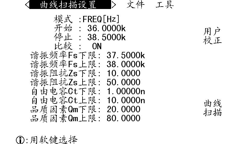
Figure 4-3: < Curve Scan Settings> Page

On the < Curve Scan Settings> page, you can configure the following main parameters:

Scan Mode (Mode)

Scan Conditions (Start, End)

Comparison: ON or OFF

Comparison Criteria Settings:

Includes: lower limit of resonant frequency Fs, upper limit of resonant frequency Fs, lower limit of resonant impedance Zs, upper limit of resonant impedance Zs, lower limit of free capacitance Ct, upper limit of free capacitance Ct, lower limit of quality factor Qm, and upper limit of quality factor Qm.

4.4.1 Scan Mode (Mode)

The default scan mode for the Impedance analyzer is “Frequency [Hz].”

4.4.2 Scan Conditions (Start, End)

The “Start Range” menu option is used to set the starting conditions for a curve scan.

The “End Range” menu option is used to set the end conditions for a curve scan.

How to set start or end conditions:

When the cursor is positioned on the start field or end field: Use the numeric keypad to select the number you want to enter. After entering the number, press the Enter key or the “Unit” soft key to confirm.

4.4.3 Setting Comparison Conditions

When “Compare” is set to OFF, the instrument will not perform a comparison after completing the scan and measurement.

When “Comparison” is set to ON, after the instrument completes its scan and measurement, it will compare the corresponding parameters against the upper and lower limits.

How to enter the upper and lower limits:

Enter the numbers using the numeric keys, then select the corresponding units from the soft-key area on the right side of the screen to complete the input of the upper and lower limits.

4.5 Curve Scan Display

Press the [LCRZ] key to enter the < Curve Scan Display> page, as shown in the figure below.

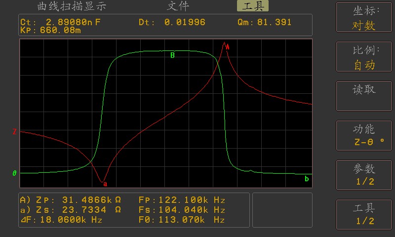
Figure 4-4: < Curve Scan Display> Page

The < Curve Scan Display> page automatically scans the device under test at frequencies of 101201,401, or 801-point frequency, in either linear or logarithmic mode, with the test conditions incrementing sequentially. It dynamically displays on the LCD screen the response curves of the device’s primary and secondary parameters as the test conditions change, and the measurement results for any point within the scan range can be read directly from the screen. It also displays the maximum and minimum measured values of the primary and secondary parameters for the device within the scan range, along with the corresponding test conditions.

Note: After the user has set the scan conditions, they must press the [TRIGGER] button on the front panel to start the scan.

4.5.1 Display of Scan Results

The “Curve Scan Display” page primarily shows the following:

Free Capacitance Ct

Free Capacitive Loss Dt

Quality Factor Qm

Planar Electromechanical Coupling Coefficient Kp

Point A: Anti-resonance impedance Zp and anti-resonance frequency Fp

Point a: Resonant impedance Zs and resonant frequency Fs

△F = anti-resonance frequency Fp – resonance frequency Fs

F0 = (anti-resonance frequency Fp + resonance frequency Fs)/2

Variable Resistor R1

Dynamic Inductor L1

Variable Capacitor C1

The maximum value of θ and the frequency corresponding to that maximum value

The minimum value of θ and the frequency corresponding to that minimum value

4.5.2 File Management (Files)

File Management

Press this soft key to access the file management page, where you can save the configured parameters as a file for future use.

Screenshot

Press this soft key to copy the information on the screen to a USB flash drive.

4.5.3 Common Menus for Curve Scanning

In the “Curve Scan Display” page under the Tools section, the following soft-key operations are available:

Tap this soft key to switch between “Coordinates: Logarithmic” and “Coordinates: Linear.”

Linear Coordinates: The scan increments linearly, and the vertical coordinates are also distributed linearly.

Logarithmic coordinates: The scan increments in a logarithmic scale with base 10, and the vertical axis is also distributed in a logarithmic scale with base 10.

Tap this soft key to toggle between “Scale: Auto” and “Scale: Locked.”

At this point, the system will automatically adjust the display scale of the curve during each scan to fit the curve display area.

Lock the display scale of the system lock curve at this point; each scan will plot the curve using the locked scale and the maximum and minimum values.

Note: It is generally recommended that users select “Auto” for the ratio.

The “Read This Area” feature allows users to view the measurement results for each scan condition.

When you press the “Read” button, “Read” appears in this area, indicating that the system is currently in data-reading mode. At this point, the screen appears as shown in the figure below:

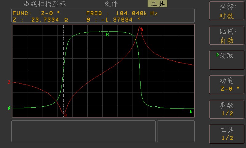
Figures 4–5: Reading Frequency and Impedance

FUNC: Z-θ. The current measurement function.

FREQ: 36.55 kHz—the frequency point corresponding to the current dashed line.

Z: 6.09472 Ω—the principal parameter value corresponding to the current dashed line.

θ: -9.01012. The value of the secondary parameter corresponding to the current dashed line.

Special Note: To view the measurement results for each condition point, follow these steps: Use the arrow keys on the panel. The [↓] key moves quickly toward the high end (right); the [↑] key moves quickly toward the low end (left); the [→] key moves one condition point at a time toward the high end (right); [←] moves one condition point at a time toward the lower end (left); Press the “Read” key once more to exit read mode.

To cycle through the functions, press this button repeatedly to switch between the Z-θ, R-X, and G-B functions. It is generally recommended to select the Z-θ function.

Parameter 1/2: Press this button, and the screen will display: dynamic resistance R1, dynamic inductance L1, dynamic capacitance C1, θmax and the corresponding frequency, as well as θmin and the corresponding frequency.

Tool 1/2: Press this key to display the Speed, Curve Mode, Number of Points, Scan Settings, Parameter 2/2, and Tool 2/2 menus in the soft-key area.

Press this button to switch between scan speeds: FAST, MED, and SLOW.

At this point, it takes FAST 5 ms to scan a single point.

At this point, it takes MED 15 ms to scan a single point.

At this point, SLOW takes 70 ms to scan a single point.

Curve Mode Press this button to switch between Curve A, Curve B, and Curve A+B

Curve A: Displays only the main parameters during scanning

Curve B: Displays only secondary parameters during scanning

Curve A+B: Displays both primary and secondary parameters simultaneously during scanning.

To switch between scan codes 101201, 401, and 801, press this button.

Number of scan points: This refers to the number of points in a step-by-step scan within the start and end conditions. The more scan points you select, the more precise the resulting image will be, but the scan will take longer.

Scan Settings Press this button to quickly access the scan settings page

Parameter 2/2: Press this key to display the following parameters on the screen: free capacitance Ct, free capacitance loss Dt, quality factor Qm, the maximum values of the main parameters and the frequencies corresponding to those maximum values, as well as the minimum values of the main parameters and the frequencies corresponding to those minimum values.

Tool 2/2: Click this item to toggle the soft-key area on the screen, which will display the Coordinates, Scale, Read, Functions, Parameters 1/2, and Tools 1/2 menus.

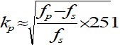
When the user selects Z-θ (frequency and impedance) as the scan parameters, the instrument automatically displays certain parameters of the ultrasonic device. The specific parameters are described below:

Static capacitance Ct: Capacitance value at 1 kHz.

Static capacitance Dt: Capacitance value at 1 kHz.

Minimum impedance Zmin and its corresponding frequency fs (point a on the screen).

Maximum impedance Zmax and its corresponding frequency fp (point A on the screen).

。

。

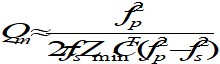
ΔF = fp – fs

4.6 LS80A HANDLER Sorting Interface

The pin layout of the HANDLER interface is shown in the figure below:

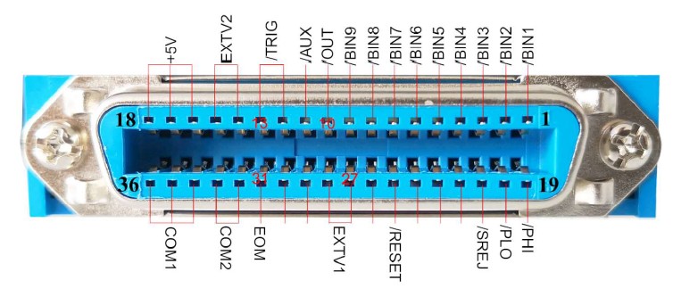
Figure 4-6 LS80A HANDLER Sorting Interface Pinout Diagram

The meanings of the HANDLER pin signals for the LS80A series instruments are shown in the table below:

Pin Number	Signal Name	Signal Type	Signal Meanings
1	/BIN1	Output	Valid signal, low active
10	/OUT	Output	Invalid signal, low active
12	/TRIG	Input	Trigger signal, active low. Triggers instrument measurement, active low. This signal is supplied externally to the HANDLER’s input.
31	/EOM	Output	Measurement complete signal, active low.
27	EXTV1	Power Supply Positive Terminal	External input power supply pin. Connect to the positive terminal of the external power supply.
36	COM1	Negative Terminal of the Power Supply	Connect to the negative terminal of the external power supply. 0V
Other			The other pins are not used in this instrument.

5. LS90A Series Impedance Analyzer Operating Guide

5.1 Instrument Front Panel

The instrument’s front panel is shown in the figure below.

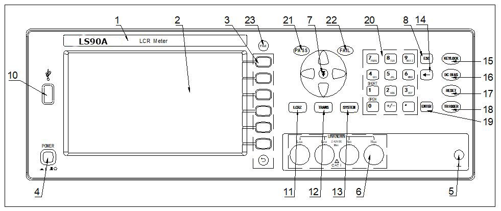
Figure 5-1 Instrument Front Panel

Brands and Models

Instrument brand, model, measurement range, etc.

LCD Display

Extra-large 800×480 dot-matrix LCD display showing setup information, measurement results, measurement conditions, and more.

Soft Keys

Six soft keys are available for selecting controls and parameters; the function of each soft key is defined to the left of it. The soft key definitions vary depending on the display page.

Power Switch (POWER)

Press this button to turn the power on or off.

Chassis When connecting the instrument to a power source Terminal

This terminal is connected to the instrument housing. It can be used for protective or shielding When connecting the instrument to a power source connections.

Test End (UNKNOWN)

Four-terminal to test terminal. Used to connect a four-terminal test fixture or test cable for measuring the device under test.

High-side current drive (Hcur);

High-side voltage sampling (Hpot);

Low-end voltage sampling (Lpot);

Low-end current drive (Lcur).

NEXT button

Quick Page-Turn Keys

ESC key

Finish entering the numbers on the numeric keypad.

To be expanded

USB Host Port

Used to connect a USB flash drive.

[LCRZ] Menu Key

Press the [LCRZ] key to go to the “Drawing Scan” page.

[SETUP] Menu button

Press the [SETUP] button to enter the “Drawing Settings” main screen.

[SYSTEM] Menu button

Press the [SYSTEM] button to access the “System Settings” page.

[←] key

The BACKSPACE key. Press this key to delete the last character of the entered value.

KEYLOCK Key

Press the [KEYLOCK] button; the [KEYLOCK] indicator will light up, indicating that the panel buttons are currently locked. Press the [KEYLOCK] button again; the [KEYLOCK] button will turn off, indicating that the keypad lock has been released. If the password function is set to “ON,” you must enter the correct password to release the keypad lock; otherwise, the keypad lock cannot be released.

When the instrument is controlled via a bus (such as USBTMC), the [KEYLOCK] button will light up. Press the [KEYLOCK] button again, and it will turn off, indicating a return to local mode and the release of the keyboard lock.

[DC BIAS] button

Reserve

[RESET] button

Keyboard Shortcuts for Capturing the Instrument Screen

[TRIGGER] key

When the instrument’s trigger mode is set to MAN (Manual), press this key to trigger the instrument to perform a test.

[ENTER] key

When entering values, press the [ENTER] key to complete data entry, confirm, and save the data displayed on the bottom line of the LCD.

When entering a filename, press the [ENTER] key to finish entering the filename, confirm it, and save the filename displayed on the bottom line of the LCD.

Number Keys

Used to enter numbers and other relevant information.

PASS LED

The test results are indicated by an LED light.

FAIL LED

The test failed due to the LED light.

5.2 Rear Panel of the Instrument

The rear panel of the instrument is shown in the figure below.

Figure 5-2 Rear Panel Diagram of the Instrument

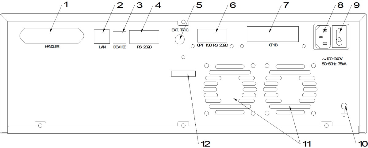
(1) HANDLER Port

The instrument uses this interface to output the results of the range comparison and the interlock signals, and also receives the “Start” signal through this interface.

(2) LAN port (optional)

Network communication interface that can be connected to a computer via an Ethernet cable.

(3) USBDEVICE Interface

The USBDEVICE interface enables a computer to control the LCR digital bridge.

(4) RS-232C Serial Interface

Serial communication interface, which allows a computer to control the instrument.

(5) EXT. TRIG Input

When the instrument’s trigger mode is set to External Trigger (EXT), this interface can be used to trigger the instrument to perform a measurement.

(6) Isolated RS-232 serial port (optional)

(7) GPIB Interface (Optional)

The GPIB interface enables parallel communication with a computer, allowing you to set up a GPIB test system.

(8) Power Outlet

AC 220V/110V input power supply connection socket.

(9) Power Switch

After plugging in the power cord, set this power switch to the “I” (ON) position, then turn on the power switch on the front of the instrument, and the instrument will begin a power-up test.

(10) When connecting the instrument to a power source post

This terminal is connected to the instrument housing. It can be used for a protective or shielding When connecting the instrument to a power source connection.

(11) Ventilation Window

Heat dissipation to maintain the instrument at its normal operating temperature.

(12) Barcode Label Area

Used for affixing instrument barcodes.

5.3 Instrument Password

Default startup password for the instrument: 2786

5.4 Drawing Settings

Press the [SETUP] main menu button to enter the < Plotting Settings> page, which is shown in the figure below.

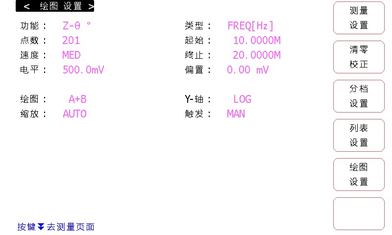
Figure 5-3: < Drawing Settings> Page

On the < Drawing Settings> page, you can configure the following main parameters:

Scan Type (Type)

Scan Condition 1 (Start, End)

Scan Conditions 2 (Function, Count, Speed, Level, Trigger, Offset)

Graph Settings (Plotting, Y-Axis, Scaling)

5.4.1 Scan Types (Types)

Move the cursor to Scan Mode (Mode Area), and the following soft keys will appear:

Frequency [Hz] Press this soft key to select the “Frequency [Hz]” scan function.

Voltage Level [V] Press this soft key to select the voltage level [V] scan mode.

Current Level [A] Press this soft key to select the “Current Level [I]” scanning mode.

Offset [V] Press this soft key to select the offset voltage mode [V] for the scan function.

Offset [A] Press this soft key to set the scan function to offset current mode [I]

Note: For the LS90A, we recommend that customers select “Frequency” as the scan type.

5.4.2 Scan Conditions 1 (Start, End)

The “Start Range” menu option is used to set the starting conditions for a curve scan.

The “End of Range” menu option is used to set the end condition for a curve scan.

How to Set Start or End Conditions:

When the cursor is positioned on the start field or end field: Use the numeric keypad to select the number you want to enter. After entering the number, press the Enter key or the “Unit” soft key to confirm.

5.4.3 Scan Conditions 2 (Functions, Number of Points, Speed, etc.)

Function: Select the parameters to be scanned; we recommend that customers select Z-

Number of Points: Set the number of scan points (101201, 401, or 801); we recommend that customers set it to 201.

Speed: Set the scanning speed (Fast, Medium, Slow); we recommend that customers select Medium.

Level: Set the scan level; we recommend that customers set it to 500 mV.

Trigger: Set the trigger mode (INT, MAN, EXT). We recommend that customers set it to MAN (manual trigger).

Offset: Set the DC offset; we recommend that customers set the DC offset to 0.

5.4.4 Graphics Settings

Plotting: You can choose to plot the primary parameter A, the secondary parameter B, or both primary and secondary parameters A and B simultaneously. We recommend selecting A+B.

Y-axis: You can choose between linear and logarithmic; we recommend selecting logarithmic (LOG).

Zoom: You can choose between “Auto Zoom” and “Lock.” We recommend selecting “Auto Zoom.”

5.5 Drawing and Scanning

Press the [LCRZ] key to enter the < Drawing Scan> page, as shown in Figure 4-5.

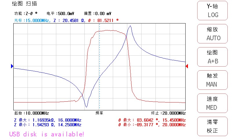
Figure 4-5: < Drawing Scan> Page

The < Plot Scan> page automatically scans the device under test at 101201,401, or 801 points, in either linear or logarithmic mode, incrementally increasing the test parameters and conditions. It dynamically displays on the LCD screen the response curves of the device’s primary and secondary parameters as the test parameters and conditions change, and the measurement results for any point within the scan range can be read directly from the screen. It also displays the maximum and minimum measured values of the primary and secondary parameters for the component within the scan range, along with the corresponding test conditions.

Note: After the user has configured the scan parameters, they must press the [TRIGGER] button on the front panel to start the scan.

5.5.1 Display of Primary and Secondary Parameter Measurements and Corresponding Conditions

The “Curve Scan Display” page primarily shows the following:

Max and Frequency: This section displays the maximum values (max) of the main parameters and their corresponding conditions.

Min and Frequency: This section displays the minimum values (min) of the main parameters and their corresponding operating conditions.

B max and Frequency: This section displays the maximum values (max) of the secondary parameters and their corresponding operating conditions.

B min and Frequency: This section displays the minimum values (min) of the secondary parameters and their corresponding operating conditions.

5.5.2 Soft-Key Menu

In the “Drawing and Scanning” page’s Tools section, the following soft-key operations are available:

Press this soft key to toggle between “Logarithmic” and “Linear” for the Y-axis coordinates.

Linear Coordinates: The scan increments linearly, and the vertical coordinates are also distributed linearly.

Logarithmic coordinates: The scan increments linearly, while the vertical axis is plotted on a logarithmic scale with base 10.

Tap this soft key to toggle between “Auto Scale” and “Scale Lock.”

At this point, the system will automatically adjust the display scale of the curve during each scan to fit the curve display area.

Lock the display scale of the system lock curve at this time.

Drawing Mode: Press this key to select a drawing method

A+B The change curves for both the primary and secondary parameters are displayed

A Display only the trend line for parameter A

B Display only the variation curve for parameter B

Trigger: Press this button to switch between trigger modes: MAN, EXT, and INT.

MAN stands for “manual trigger scan”; when the user presses the [TRIGGER] button once, the instrument performs one scan of the curve.

EXT indicates an external trigger scan; when the external interface or computer triggers once, the instrument scans the curve once.

INT stands for internally triggered scanning; after the instrument completes one full scan of the curve, it automatically proceeds to the next one.

Press this button to toggle between scan speeds: FAST, MED, and SLOW.

At this point, it takes FAST 10 ms to scan a single point.

At this point, it takes MED 50 ms to scan a single point.

At this point, it takes 166 ms for SLOW to scan a single point.

Zero Calibration

Press this button to access the zeroing and calibration page.

5.6 LS90A HANDLER Sorting Interface

The pin layout of the HANDLER interface is shown in the figure below:

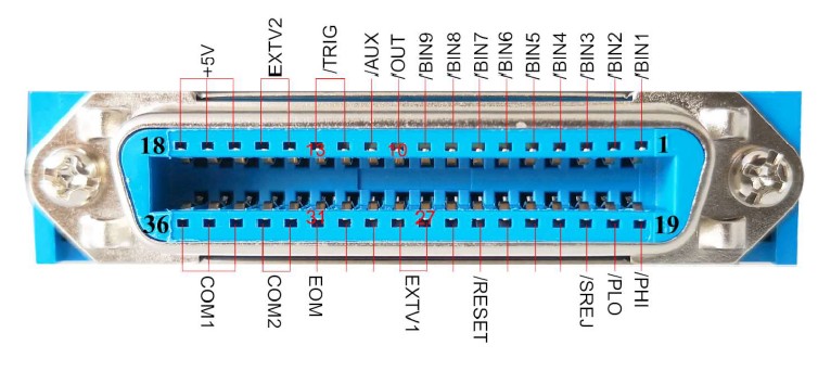
Figure 4-6 LS90A HANDLER Sorting Interface Pinout Diagram

The meanings of the HANDLER pin signals for the LS90A series instruments are shown in the table below:

Pin Number	Signal Name	Signal Type	Signal Meanings
1	/BIN1	Output	Valid signal, low active
10	/OUT	Output	Invalid signal, low active
12	/TRIG	Input	Trigger signal, active low. Triggers instrument measurement, active low. This signal is supplied externally to the HANDLER’s input.
31	/EOM	Output	Measurement complete signal, active low.
27	EXTV1	Power Supply Positive Terminal	External input power supply pin. Connect to the positive terminal of the external power supply.
36	COM1	Negative Terminal of the Power Supply	Connect to the negative terminal of the external power supply. 0V
Other			The other pins are not used in this instrument.

6. User Guide for Impedance Analysis Software

6.1 Selecting a Communication Interface and Installing Drivers (Very Important)

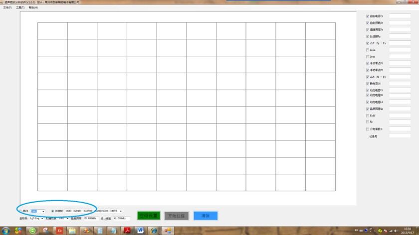
The ultrasonic impedance analysis software offers two interface options for users: an RS232C serial port and USBTMC.

For users whose computers do not have an RS232C serial port, the USBTMC communication interface is the most convenient option. Users simply need to connect the instrument to the computer using a USB cable and then install the VISARUNTIME interface driver.

(1) To select a serial port, first click the checkbox next to the serial port, then select the appropriate serial port from the drop-down list. The baud rate for the serial port is 115200.

(2) To select USBTMC, the user should first click the checkbox next to USBTMC. If the instrument’s bus mode is already set to USBTMC and the USB cable is properly connected, the analysis software will automatically detect the USBTMC communication interface; the user does not need to reselect it.

Note: If this is the first time a user is using the impedance analysis software, simply select the last port name in the port drop-down list. See the figure below. Once communication is successful, the software will automatically select the port name used for the last successful connection the next time.

Serial Port Drop-Down List:

USBTMC Interface Drop-Down List:

How to Install the USBTMC Driver:

Double-click the visa462runtime.exe file. Follow these installation steps (click the buttons circled in the order shown):

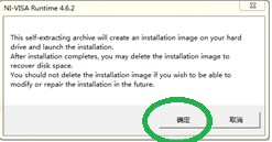
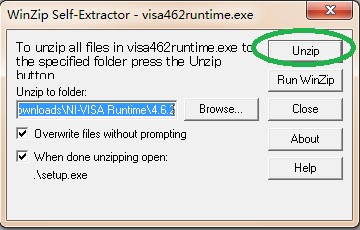
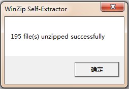
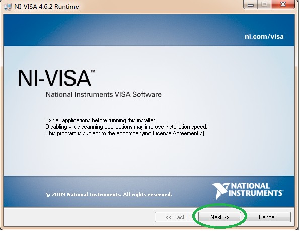
Keep clicking the “Next” button.

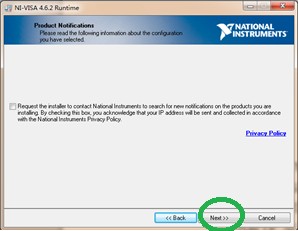
Keep clicking the “Next” button until the installation is complete.

(3) To select USBCDC, first click the checkbox next to the serial port, then select the corresponding serial port from the drop-down list.

How to Install the USBCDC Driver:

After selecting the USBCDC port on the instrument, connect the instrument to the computer using a USB cable. A dialog box will pop up on the computer asking whether to install the driver manually or automatically; select “Manual installation.” If the driver installation dialog box does not appear, go to the computer desktop, select “My Computer” (or “Computer”), right-click it, click “Properties” in the context menu to open “Device Manager,” as shown in the figure below:
Right-click the USB device recognized by the computer (the one with a yellow exclamation mark next to it), select “Update Driver Software” from the context menu, and then follow the steps shown in the figures below to install the driver:

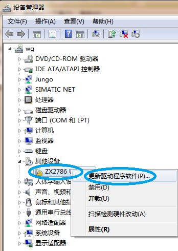
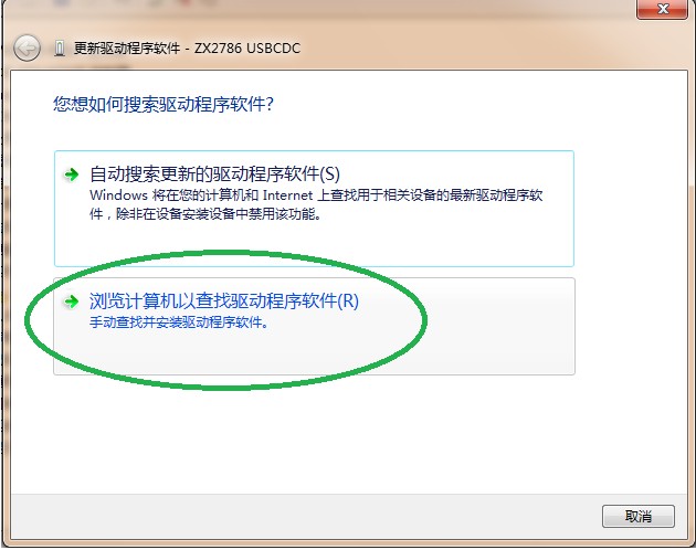
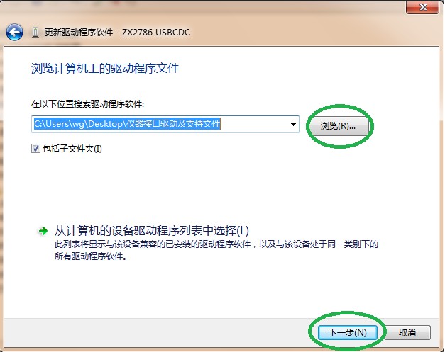
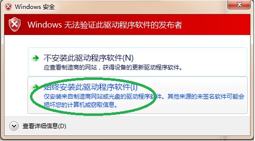
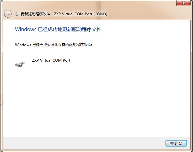
Once the driver is installed, restart your computer.

Connect the instrument to the computer using a USB cable.

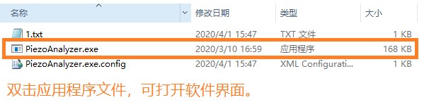
Double-click the application file on the USB drive included with our shipment to open the software on your computer, as shown in the image below.

6.2 Selecting the Coordinate System, Number of Scan Points, and Frequency Range

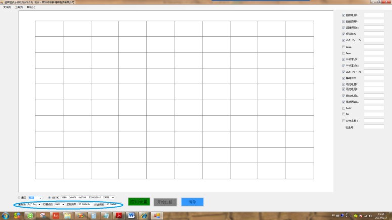
Users can select the coordinate system, number of scan points, start frequency, and cutoff frequency based on their specific analysis needs.

6.3 Synchronizing Analysis Software and Instruments

Click the “Application Settings” button to synchronize the parameters between the analysis software and the instrument.

6.4 Start scanning

Click the “Start Scan” button. The analysis software will perform measurements, analysis, and calculations based on the specified parameters—such as the coordinate system, number of scan points, start frequency, and cutoff frequency—and plot the corresponding curve. The scan results are shown in the figure below:

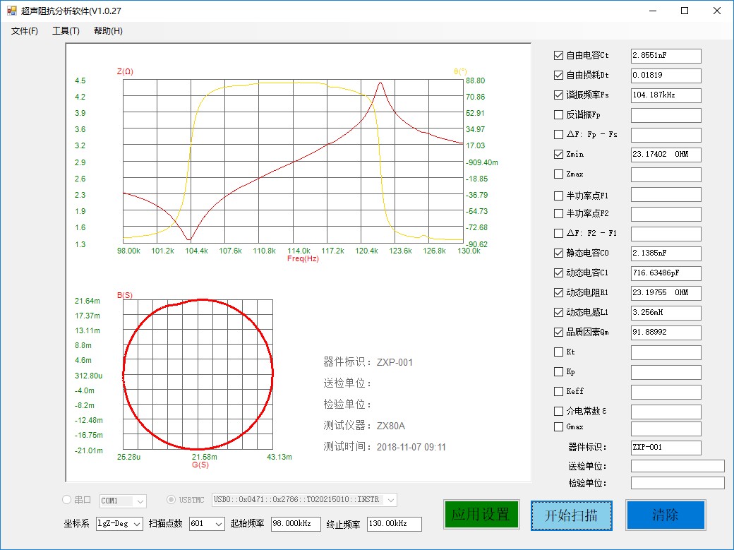
6.5 The analysis results show that

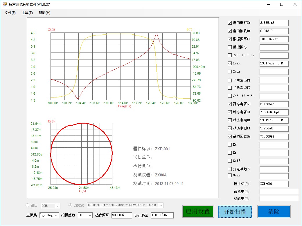
Select the corresponding parameter. Once the software has finished scanning all points, it will display the analysis results for the selected parameter.

6.6 Other Common Settings

Select “Options” from the “Tools” drop-down menu in the menu bar to open the dialog box shown below:

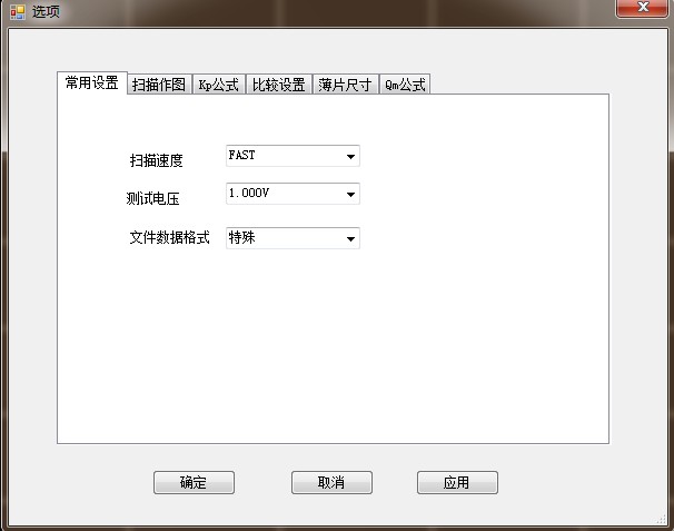
6.6.1 Common Settings

On the “General Settings” tab, you can configure the scan speed, test voltage, and file data format.

6.6.2 “Scan-to-Draw” Settings

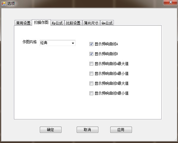
On the “Scan and Plot” settings tab, you can configure the plotting style, the frequency response curve, and how the maximum and minimum values of the frequency response curve are displayed.

6.6.3 “Kp Formula” Settings

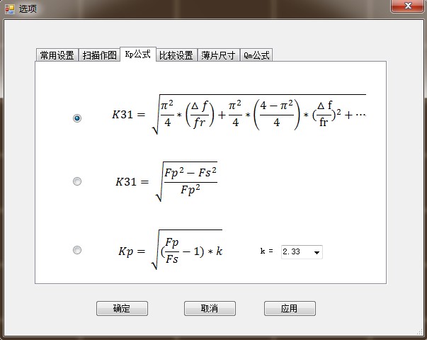
On the “Kp Formula” tab, customers can select the Kp calculation formula that best suits their needs.

6.6.4 “Comparison Settings” Tab

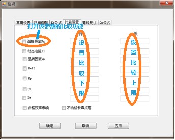
On the “Comparison Settings” tab, you can set the upper and lower limits for comparisons of resonant frequency, dynamic resistance, quality factor, Keff, Kp, Ct, and Dt, and configure either a “pass” dual-tone beep or a “fail” long beep.

6.6.5 “Slice Dimensions” Tab

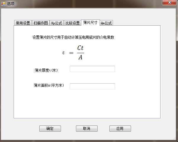
On this tab, enter the thickness and area of the wafer required to calculate the dielectric constant of the piezoelectric ceramic wafer.

In the above formula, C is the free capacitance, measured in pF; t is the thickness of the wafer, measured in mm; and A is the area of the wafer, measured in mm². This parameter applies only to piezoelectric ceramic wafers.

6.6.6 “Qm Formula” Tab

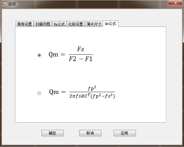
This tab is used to select the formula that Qm uses for analysis and calculations.

6.6.7 Apply or Cancel Settings

Click the “Apply” or “OK” button to apply the settings from the tab above.

If you click the “Cancel” button, the above settings will not take effect.

6.7 Saving and Loading Settings

Click “Save Settings” under the “File” menu to save all of the software’s current settings to a file.

Click “Load Settings” under the “File” menu to load the settings saved in the file into the software.

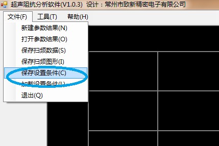
6.8 Saving Data and Images

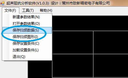
Click “Save Sweep Data” under the “File” menu to save the data from this scan to a file.

Click “Save Sweep Image” under the “File” menu to save the graph of the current scan as an image file.

6.9 Saving Parameter Results

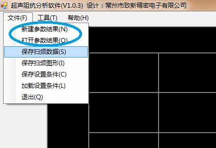
“New Parameter Results” is used to create a new file to save the various parameters obtained from the scan analysis (such as Ct, Dt, etc.; note that parameters must be selected in order to be saved).

“Open Parameter Results” is used to open a file and view the saved parameter results.

7. Frequently Asked Questions and Solutions

7.1 Software Installation and Operation Issues

(1) The software won’t open properly

Generally, you can open and run the analysis software by double-clicking the “PiezoAnalyzer.exe” application file (as shown in the figure above; it is typically 133 KB in size).

If the analysis software does not open when you double-click the application file, you can try the following solutions:

Turn off the antivirus software on your computer;

Install the Windows patch package “ . NET Framework 2.0 or later”; this applies to older versions of Windows XP.

Install the VISA RUN TIME 462 Driver Package

You can download this driver package from the link in My Cloud: https://pan.baidu.com/s/1TC0xMsiWMjJqnK0jwBw2Gw

Extraction code: 669i

Once the installation is complete, you’ll need to restart your computer.

If you are still unable to open the software after following the steps above correctly, we recommend trying it on a different computer.

(2) Failed to connect to the interface

Users who use the serial port can resolve this issue by following these steps:

a. Check whether the bus mode on the instrument is set to “RS232C” and whether the baud rate is set to 115200;

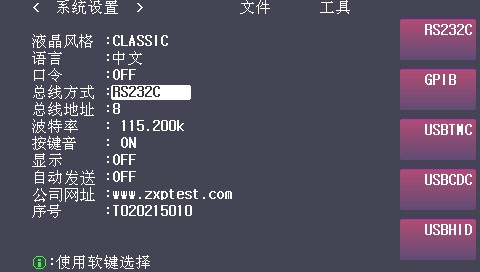
b. Check Device Manager to see if the serial port card and serial port driver are installed correctly;

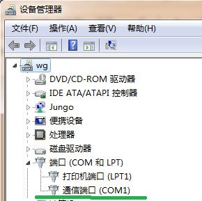
c. Check whether the serial cable is connected properly.

d. Restart the instrument and the software.

Users of USBTMC can resolve this issue in the following ways:

a. Check whether the instrument’s bus mode is set to “USBTMC”;

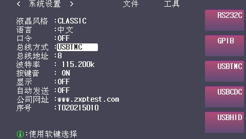
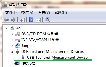
b. Check in Device Manager to see if the USBTMC device is recognized properly and if the device driver is installed correctly;

If there is a yellow “?” next to the device name, you need to unplug and replug the USB device, then reinstall the VISARUNTIME driver, or right-click the device name and select “Manually Install Driver”;

c. Check to see if the USB cable is working properly.

d. Restart the instrument and the software.

7.2 Analyzing Software Scan Issues

(1) The following graph appears for the admittance circle:

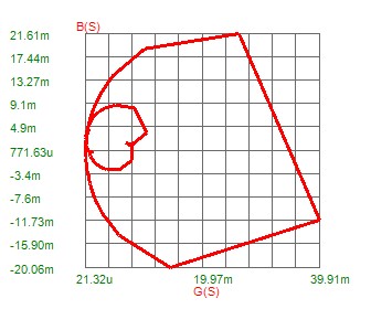
Possible reasons are as follows:

a. The scan frequency range is too wide. For example, if the resonance frequency is 40 kHz and the anti-resonance frequency is 43 kHz, setting the scan range to 1 kHz–45 kHz will cause the problem described above. The solution is to narrow the scan range; for example, set the frequency range to 39 kHz–45 kHz.

b. The device has a very high Qm value; the higher the Qm, the narrower the bandwidth. The solution is to select a higher number of scan points.

(2) The scanned image is as follows:

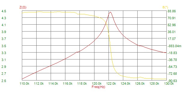
The scan frequency did not include the resonance frequency.

Solution: Slightly lower the starting frequency.

1. 1: LS70A Series Impedance Analyzer Product Models and Specifications

Model Specifications	LS70A_200k	LS70A_500k	LS70A_1M
Frequency Range	20 Hz–200 kHz	20 Hz–500 kHz	20 Hz–1 MHz
Scan Parameters	R-X, Z-θ, Y-θ, G-B	R-X, Z-θ, Y-θ, G-B	R-X, Z-θ, Y-θ, G-B
Basic Accuracy (Subject to the accuracy table)	0.05%	0.05%	0.1%
Measurement Speed (equivalent to 400 points)	4 seconds per item (instrument scan)	4 seconds per item (instrument scan)	4 seconds per item (instrument scan)
Frequency Accuracy	1 mHz	1 mHz	1 mHz
Phase resolution	0.01.	0.01.	0.01.
Impedance Range	0.01 mΩ to 99.99 MΩ	0.01 mΩ to 99.99 MΩ	0.01 mΩ to 99.99 MΩ
Interface	RS232C, USB CDC, USB TMC, Handler, GPIB (optional)	RS232C, USB CDC, USB TMC, Handler, GPIB (optional)	RS232C, USB CDC, USB TMC, Handler, GPIB (optional)
Suitable Occasions	Powered ultrasonic equipment testing, ultrasonic cleaning, ultrasonic welding, ultrasonic medical applications	Powered ultrasonic equipment testing, ultrasonic cleaning, ultrasonic welding, ultrasonic medical applications	Mass Inspection of Production Lines for Piezoelectric Ceramics Below 1 MHz

2. 2: LS80A Series Impedance Analyzer Models and Specifications

Model Specifications	LS80A_2M	LS80A_5M
Frequency Range	20 Hz–2 MHz	20 Hz–5 MHz
Scan Parameters	R-X, Z-θ, Y-θ, G-B	R-X, Z-θ, Y-θ, G-B
Basic Accuracy (Subject to the accuracy table)	0.1%	0.1%
Measurement Speed (equivalent to 400 points)	4 seconds per item (instrument scan)	4 seconds per item (instrument scan)
Frequency Accuracy	1 mHz	1 mHz
Phase resolution	0.01.	0.01.
Impedance Range	0.01 mΩ to 99.99 MΩ	0.01 mΩ to 99.99 MΩ
Interface	RS232C, USB CDC, USB TMC, Handler, GPIB (optional)	RS232C, USB CDC, USB TMC, Handler, GPIB (optional)
Suitable Occasions	Production and Testing of Piezoelectric Ceramics Below 2 MHz	Production and Testing of Piezoelectric Ceramics Below 5 MHz

3. 3: LS90A Series Impedance Analyzer Models and Specifications

Model Specifications	LS90A_5M LS90A_10M LS90A_15M LS90A_20M LS90A_25M
Frequency Range	LS90A_5M: 20 Hz – 5 MHz LS90A_10M: 20 Hz – 10 MHz LS90A_15M: 20 Hz to 15 MHz LS90A_20M: 20 Hz to 20 MHz LS90A_25M: 20 Hz to 25 MHz
Scan Parameters	R-X, Z-θ, Y-θ, G-B
Basic Accuracy (Subject to the accuracy table)	0.1%
Measurement Speed (equivalent to 400 points)	4 seconds per item (instrument scan)
Frequency Accuracy	10 mHz
Phase resolution	0.01.
Impedance Range	0.01 mΩ to 99.99 MΩ
Interface	RS232C, USB CDC, USB TMC, Handler, GPIB (optional)
Suitable Occasions	Production and Testing of High-Frequency Piezoelectric Ceramic Devices

Photometric, Colorimetric, and Safety Performance Testing Solutions for LEDs

Goniophotometer System: LSG-6000, LSG-1890B, or LSG-1800ACCD

Spectroradiometer & Integrating Sphere Test System: LPCE-2 or LPCE-3

LED Life Maintains a Test System in Accordance with LM-84: LEDLM-84PL

Photobiological Radiation Safety Test System: EN 62471-C or EN 62471-P

Lamp Start, Run-up Time, and Flicker Test System: LSRF-3 and LSP-500VARC-Pst

LED Power Driver Testers: LS2090, M9822, and LSP-500VARC

IK Level Tester | Spring Hammer Impact Tester: IK07-10, IK01-06

Electrodynamic Vibration Generator System: LVD-100KG-6D

Electrical Safety Testers: LS9955, ZRS-3H, ZY-3, TTC-1

Environmental Chamber Test Solution for LED Luminaires

Waterproof Test for IPX5 and IPX6: JL-56

Dustproof Testing Machine for IP5X and IP6X: SC-015

High- and Low-Temperature and Humidity Chamber: GDJS-015B

Salt Spray Test Machine: YWX/Q-010

UV Lamp Aging Test Chamber: UV-263LS

Xenon Lamp Aging Test Chamber: XD-80LS

Ozone Test Chamber: OTC-150A

Sulfur Dioxide Test Chamber: SQ-010

EMC and EMI Test Solutions for CFL and LED Luminaires

EMI Test System: EMI-9KB or EMI-9KA

Electrostatic Discharge Simulator: ESD61000-2

EFT Immunity Measurement: EFT61000-4

Surge Generator: SG61000-5

Voltage Dips and Interruptions Generator: CSS61000-11

Ring Wave Generator: RWG61000-12

www. Lisungroup.com

Patents Filed

All Rights Reserved by Lisun Group

Subject to Change Without Notice